How Campaign Contributions Predict U.S. Presidential Nominations: Logistic Regression

With election season in full swing, I am unfortunately becoming increasingly obsessed with the presidential race, and I thought it would be a good exercise to play with some data on U.S. politics. I collected data from the Federal Election Commission (“FEC”) and focused on the question of what factors related to campaign contributions, given the available data, are most predictive of who wins each party’s nomination.

I explored the presidential nominations for the Republican and Democratic primaries from 1992 through 2016.

Election	Candidate	Total_contributions	Pct_Individuals	Pct_Committees	Pct_Self	Republican	Pres_Incumbent	Nominee
2008	McCain, John S	45457558	0.888827589	0.01223907	0	1	0	1
2012	Romney, Mitt	58158320	0.993713598	0.006286402	0	1	0	1
2016	Trump, Donald J.	19405217	0.337897636	0	0.661619215	1	0	1
2016	Clinton, Hillary Rodham	115563929	0.94	0.01	0	0	0	1
2008	Obama, Barack	113003997	0.99	0	0	0	0	1
2004	Kerry, John	31588031	0.77	0	0.12	0	0	1
2000	Bush, George W.	93438370	0.97	0.02	0	1	0	1
2000	Gore, Al	38509532	1	0	0	0	0	1
1996	DOLE, ROBERT J	37622728	0.96	0.04	0	1	0	1
1992	CLINTON, WILLIAM JEFFERSON	5605038	1	0	0	0	0	1
2012	Obama, Barack	129875853	0.77	0	0	0	1	1
2004	Bush, George W.	166117902	0.98	0.02	0	1	1	1
1996	CLINTON, WILLIAM JEFFERSON	39155844	1	0	0	0	1	1
1992	BUSH, GEORGE HW	17723002	1	0	0	1	1	1
2012	Gingrich, Newt	13118932	0.994418478	0.005534225	0	1	0	0
2008	Paul, Ron	31159463	0.997441806	0.00062558	0	1	0	0
2016	Paul, Rand	11519438	0.824962045	0.003610395	0	1	0	0
1992	LAROUCHE, LYNDON H JR	487224	1	0	0	0	0	0
2000	Bradley	37961904	0.99	0	0	0	0	0
2012	Paul, Ron	26864507	0.980603347	0	0	1	0	0
2000	LaRouche	2836550	1	0	0	0	0	0
2016	Webb, James Henry Jr.	764992	0.99	0.01	0	0	0	0
2008	Cox, John H	1191935	0.020569897	0	0.978966138	1	0	0
2004	Moseley Braun	620314	0.94	0.06	0	0	0	0
2012	Pawlenty, Timothy	5267486	0.955758149	0.025462826	0	1	0	0
2000	Hatch	3154390	0.85	0.06	0	1	0	0
2008	Brownback, Samuel Dale	4624401	0.844470067	0.011823516	5.98E-06	1	0	0
1992	FULANI, LENORA B	1477768	1	0	0	0	0	0

In the original data, the rate of nominations is only 13%, indicating that only about 1 out of every 10 candidates wins the nomination. Given this low nomination rate, I took a retrospective design approach, sampling 14 nominees and 14 random non-nominees from the pool of total candidates during these years. The data set contains the following variables:

• Total Contributions: Total dollar contributions to a candidate’s campaign, adjusted for inflation to 2016 dollars,
• Pct_Individuals: Percentage of total contributions to a candidate’s campaign that came from individuals donations,
• Pct_Committees: Percentage of total contributions to a candidate’s campaign that came from Political Action Committees,
• Pct_Self: Percentage of total contributions to a candidate’s campaign that were self-funded,
• Pres_Incumbent: An indicator variable in which 1 represents a presidential incumbent, and 0 represents a non-incumbent,
• Nominee: The response variable indicating whether a candidate ultimately received their party’s nomination for the presidential election.

A summary of these data is as follows:

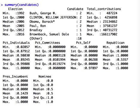
The summaries confirm that we have an equal proportion of nominees and non-nominees in this sample. Total_contributions have quite a wide range from a minimum of almost $500k to a maximum of $166 Million, with a mean of about $38 Million. The funding sources summaries show that most campaigns are funded primarily through individual donations, with a small proportion funded through PACs, and a small proportion of self-funded campaigns.

Plots of these data are:

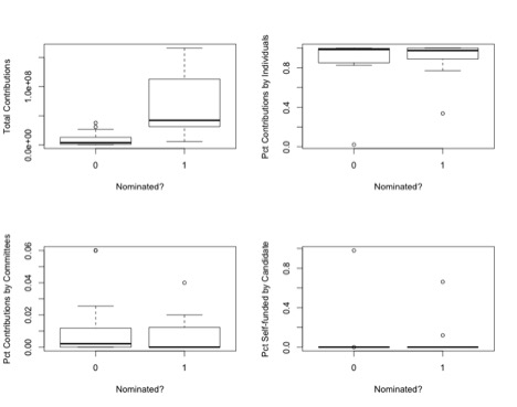
One thing that jumps out in the box plots that split Total Contributions by Nomination is that the differences between the lower levels of contributions and the higher levels are steep, perhaps multiplicative. Let’s create a variable logContributions, the natural log of Total Contributions, and plot it.

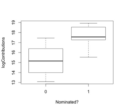
The plot of logContributions seems more reasonable. Comparing the plots of these 4 predictors, it seems that logContributions likely has the most predictive potential, whereas there appears to be little in the way of mean differences for the variables Pct_Individuals, Pct_Committees, and Pct_Self.

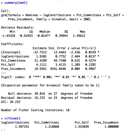
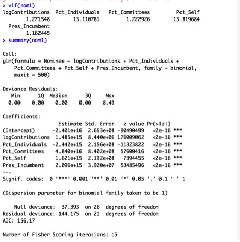
Let’s fit a logistic regression model based on all the predictors mentioned above. The output is as follows:

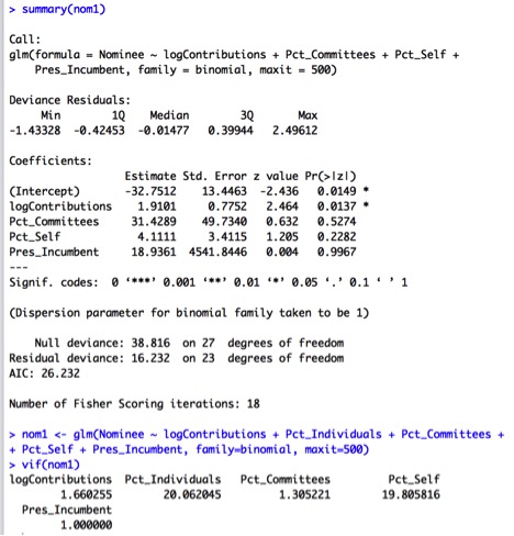
Only the logContributions variable has a significant p-value for its individual Wald test, while those of the other predictors are quite high. This suggests we should consider simplifying our model. This notion is further confirmed by the VIF values of around 20 for Pct_Individuals and Pct_Self, indicating some collinearity between the two variables. For now, I’ll remove the Pct_Individuals variable, which has the highest VIF, and re-run the model.

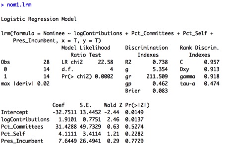
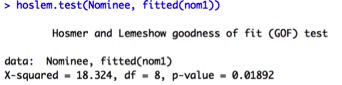
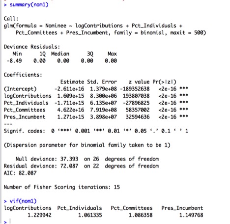
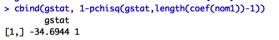
The overall model is significant with a Likelihood Ratio of 22.58 on 4 degrees of freedom, with a small p-value of 0.0002. Indeed, the VIF values look better now; however, logContributions is still the only significant variable in the model, suggesting further simplification should be considered. Somer’s D is a high 0.913, indicating excellent separation. However, the Hosmer and Lemeshow test shows that there is a lack of fit of the data within this model, with a small p-value:

When we plot the Pearson residuals, we see there is a clear outlier: #10, Bill Clinton from the 1992 election cycle:

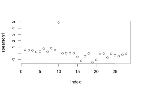
I will remove this data point and re-fit a logistic regression model to the new data set. This yields the following output:

Surprisingly, all of the predictors appear to be highly significant now. However, the VIF of Pct_Individuals and Pct_Self are both higher than 10, so I will remove the higher one, Pct_Self and re-fit a model.

While the Wald tests for each individual predictor appear to be highly significant, looking at the Likelihood Ratio Test to test overall significance of the model, we find that the model overall is not significant, with a p-value of 1:

We should look at model selection techniques to see if simplifying the model will help. Here is output from Best Subsets:

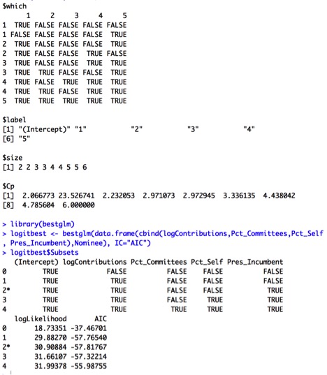
The output suggests that using only logContributions and Pres_Incumbent, or even logContributions alone, might be sensible. We therefore fit a new model using these predictors:

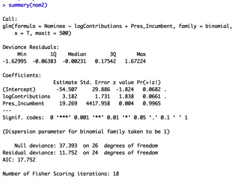
In this model, the Pres_Incumbent predictor is not significant, so I will re-fit the model using only the logContributions predictor:

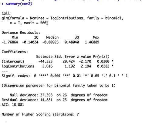
The logContributions model is now more significant, with a lower Wald Test p-value of .028.

The LR test is highly significant as well, with LR = 22.51 on 1 degree of freedom, and a p-value of less than .0001. The Somer’s D value shows excellent separation at 0.912. Also, the Hosmer-Lemeshow test shows that the model fits the data very well, with a p-value of 0.9733:

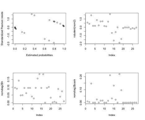
The Diagnostic plots for this model do not indicate any obvious problems. It seems that taking out Bill Clinton’s 1992 run was indeed helpful:

Now let’s look at a classification table for this model:

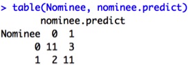
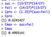
Roughly 82% of the candidates were correctly classified using this model (22 out of 27 candidates). This is much higher than either the Cpro or Cmax rates, which are 62% and 50%, respectively:

A plot of the predicted separations is:

The real-life separations would show all of the index values less than 15 to be on the nominated side, while those 15 and above would be on the non-nominated side. This looks like a fairly good plot, under the circumstances.

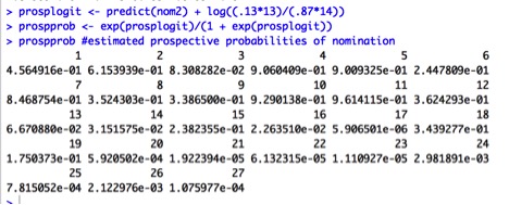
Recall that we used a retrospective approach for this study. We can obtain prospective probabilities by adjusting the Constant using prior probabilities for nomination, which are:

13% Nominated

87% Not nominated.

The results are:

 

In this post, I tried to predict Presidential Primary nominations using data related to campaign finance. What we found is that overall logged Total Contributions is a good predictor of whether a candidate receives the nomination. Most of the other predictors we tried to model on (including proportions of various funding sources, incumbency, and party affiliation) were not predictive, and I confirmed this through visual plots as well as model selection techniques. Ultimately, the simplest model won out. To further improve the model, I might have to look at other aspects of campaigns and political careers, but at this time, I will consider the final model, that based on the log of Total Contributions, to be the best choice.

 

Data Source:

Federal Election Commission, Campaign Finance Statistics (1992-2016). Presidential Candidate 12-Month Data Summaries [Data file]. Retrieved from http://www.fec.gov/press/campaign_finance_statistics.shtml.